Understanding the Core Concepts of Deep Learning with MIT 6.S191

🧠 The Building Block: Perceptron

The perceptron is the simplest type of artificial neuron. It's modeled after biological neurons and takes weighted inputs, adds a bias, and passes the result through an activation function.

Forward propagation :
for a single perceptron can be written as:

$$z = \sum_{i=1}^{n} w_i x_i + b$$ $$a = \phi(z)$$

Where:

• $x_i$ are the input features
• $w_i$ are the weights
• $b$ is the bias
• $\phi$ is the activation function
• $a$ is the output of the neuron

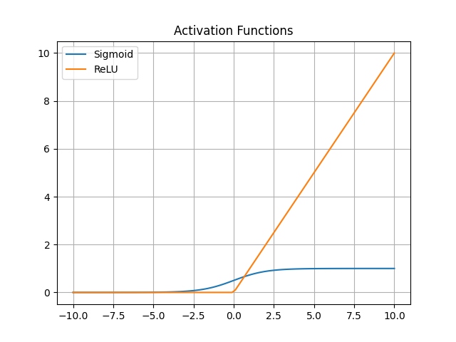
Activation functions introduce non-linearity, such as:

• Sigmoid:

$$\sigma(z) = \frac{1}{1 + e^{-z}}$$

• ReLU:

$$ReLU(z)=max⁡(0,z)$$

🕸️ Expanding the Web: Neural Networks

A neural network consists of layers of neurons. Each hidden layer performs a transformation on its inputs using dense connections (fully connected layers).

$$a(l) = \phi(W^{(l)} a^{(l-1)} + b^{(l)})$$

Where

• $l$ is the layer index
• $a^{(l)}$ is the activation of layer $l$
• $\phi$ is the activation function

📉 Loss Functions: Measuring the Error

The loss function quantifies the difference between predicted and true values. Common types include: Mean Squared Error (MSE):

$$L = \frac{1}{n} \sum_{i=1}^{n} (y_i - \hat{y}_i)^2$$

Cross-Entropy Loss (for classification):

$$L= -\sum y \log(\hat{y})$$

🔄 Backpropagation: The Learning Engine

Backpropagation is the process that allows the network to learn by updating weights based on the loss gradient.

It works by applying the chain rule from calculus, moving layer by layer from output to input.

🧠 Error propagation:

For layer $l$:

$$\delta^{(l)} = \left(W^{(l+1)}\right)^T \delta^{(l+1)} \odot \phi'\left(z^{(l)}\right)$$

For weights update:

$$W^{(l)} := W^{(l)} - \eta \cdot \frac{\partial L}{\partial W^{(l)}}$$

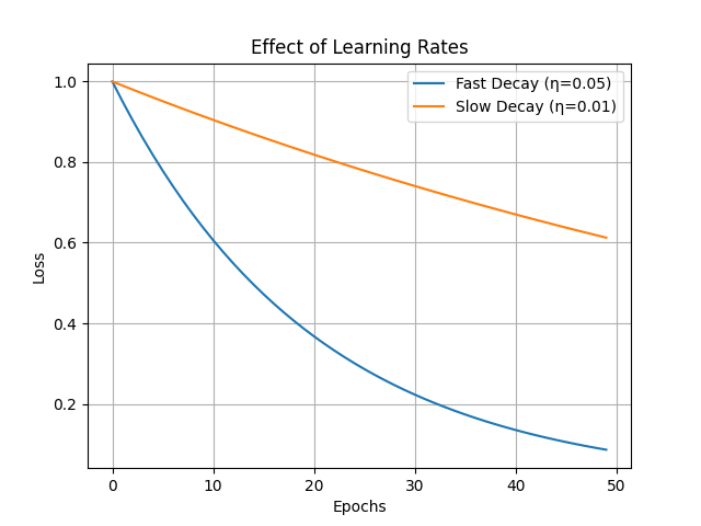
🎯 Optimization: Gradient Descent

We minimize the loss using gradient descent, which updates weights to reduce the error:

$$w := w - \eta \frac{\partial L}{\partial w}$$

Where $\eta$ is the learning rate.

Variants include:

• Stochastic Gradient Descent (SGD): uses a random mini-batch
• Mini-Batch Gradient Descent: faster, uses subset of data
• Adaptive methods: e.g., Adam optimizer

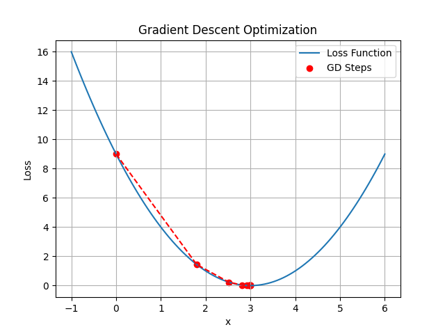
📉 Visualizing Gradient Descent

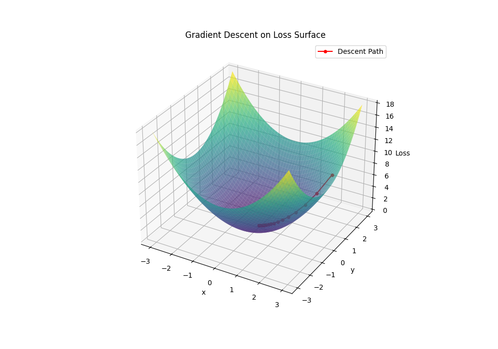
This graph shows how gradient descent minimizes a loss function: This One shows a 3d like view:

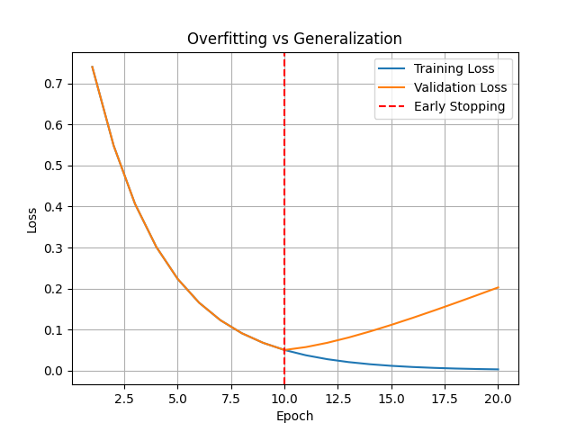
🧩 Generalization and Overfitting

A network that memorizes training data but performs poorly on new data is said to overfit.

🔧 Regularization Techniques:

• Dropout: Randomly deactivates neurons during training • Early stopping: Halts training when validation loss stops improving

🧭 Final Thoughts

This MIT 6.S191 session was a deep dive into the fundamental mechanics of deep learning. From perceptrons to adaptive learning and generalization, it laid the groundwork for building intelligent systems. Stay tuned for more as I continue my journey through this series and dive into more advanced topics like convolutional networks, sequence models, and more!

👨‍💻 If you want to learn along, check out: MIT 6.S191 Intro to Deep Learning

---

Written by Breye.